wrfplot - Plot WRF Model Output Straight from the Command Line
Why wrfplot?
If you run Weather Research and Forecasting (WRF) model, you already know that running the model is only half the job. The other half is making sense of the wrfout file. Though WRF output is a simple NetCDF file, plotting even a few variables requires you to install a bunch of software and libraries, read through lot of documentation and write your own scripts. Python has excellent modules such as wrf-python, xarray, matplotlib and cartopy to deal with WRF data. However, setting these up and getting a decent looking map out of them is a tedious process, especially for someone who just wants to see the forecast.
I faced the same issue for years. Every time I wanted a small change in the final plot (a different level, a different colour scheme, one more variable), I ended up opening the same old code base and tweaking a few lines here and there. After doing this again and again, I started looking for a command line application where I could just pass options and get the common WRF forecast images. I could not find any. Therefore, I created one and named it wrfplot.
wrfplot is free and open source (GPL v3). The source code is at https://github.com/wxguy/wrfplot and the documentation lives at https://wxguy.in/wrfplot. At the time of writing this post, the latest version is 3.2.0.
What Can it Do?
In short, you give it a wrfout file, tell it which variables you want and where to save the images. That’s all. wrfplot takes care of the rest. Here is what it supports at the moment:-
- 40 diagnostic variables, both surface (MSLP, 10m winds, 2m temperature, RH, dew point, CAPE, CIN, reflectivity, precipitation, cloud cover, helicity etc.) and upper air (winds, temperature, RH, vorticity, omega, theta-e, streamlines etc.)
- Upper air variables at standard levels of
925,850,700,600,500,400,300and200hPa or any level of your choice - Custom colour maps and contour levels
- Animated GIF of all the time steps
- Works on Linux, Windows and macOS
The main use case for me is to include it as part of WRF model run framework so that all the images are plotted immediately after the model run is completed. The other use case is to produce publication quality 2D maps without much tweaking.
Install wrfplot
There are three ways to install wrfplot. Choose whichever suits you.
Using Conda (Recommended)
Support for all platforms is provided through conda-forge. If you already have Miniconda or Anaconda installed, I would recommend creating a separate environment rather than installing into base:
1
2
conda create -n wrfplot -c conda-forge wrfplot
conda activate wrfplot
If you are wondering why I prefer conda, I have explained my reasons in my earlier post on setting up Python for Atmospheric, Ocean and Climate Sciences. wrf-python, cartopy and netcdf4 all have compiled libraries underneath and conda handles them much better than anything else.
Using pip
The package is also available on PyPI:
1
pip install wrfplot
There is no ready made wheel of
wrf-pythonfor Linux or Windows on PyPI. On a fresh Python environment,piptries to compile it from source, which requiresnumpyand a Fortran compiler to be already in place. In most cases it fails. Therefore, use conda method mentioned above unless you know what you are doing. It will save you a lot of time.
Standalone Installer (Linux and Windows)
Since it is intended to be used as a command line application, it is also distributed as a standalone installer. No Python, no conda and no admin rights required. Go to https://github.com/wxguy/wrfplot/releases and download the latest release. For Windows, download wrfplot-windows-64bit.exe and install it like any other Windows setup file. For Linux, download wrfplot-linux-64bit.run and execute it (assuming it is downloaded at ~/Downloads):
1
bash ~/Downloads/wrfplot-linux-64bit.run
The installer copies the application to ~/.wrfplot, links the executable in ~/.local/bin and adds it to your PATH. Restart your terminal once the installation is completed.
The Linux installer requires at least Ubuntu 20.04 or Red Hat 8.x (or equivalent Distros) and works only on 64bit machines.
Check Installation
Whichever way you choose, check if the installation is successful by typing the following command:
1
wrfplot --version
which should print the version number. You can also see all the available options with wrfplot --help.
List Supported Variables
The first step is to know which variables wrfplot can plot. The application accepts variable names only in a certain format and hence you should have a look at the list first:
1
wrfplot --list-vars
This will print a long list. A part of it is shown below:
1
2
3
4
5
6
7
8
9
10
11
12
13
****    ****    ****    ****    ****    ****    ****
Variables starting with 'u_' are upper air variable availabe at 925, 850, 700, 600, 500, 400, 300 and 200 hPa heights...
****    ****    ****    ****    ****    ****    ****

Variable "slp"   --> Mean Sea Level Pressure (hPa)
Variable "winds"   --> Surface (10M) Wind Speed and Direction (Kt)
Variable "rh2"   --> 2m Relative Humidity (%)
Variable "T2"   --> 2m Temperature (°C)
Variable "mcape"   --> CAPE Maximum ($J kg^{1}$)
...
Variable "u_winds"   --> Wind Speed and Direction (Kt)
Variable "u_cin"   --> Convective Inhibition ($J kg^{1}$)
Variable "u_cape"   --> Convective Available Potential Energy ($J kg^{1}$)
The name within quotes such as "rh2" is the short name you will be using in all the commands. All the variables starting with u_ are upper air variables and the rest are surface variables. The complete list is also available at https://wxguy.in/wrfplot/variables/.
Plot Surface Variable
To plot any variable, there are three minimum arguments required. They are:-
--vars: Name of variable(s) to plot--input: Path towrfoutNetCDF file--output: Path to directory where images are to be saved. It will be created if it does not exist
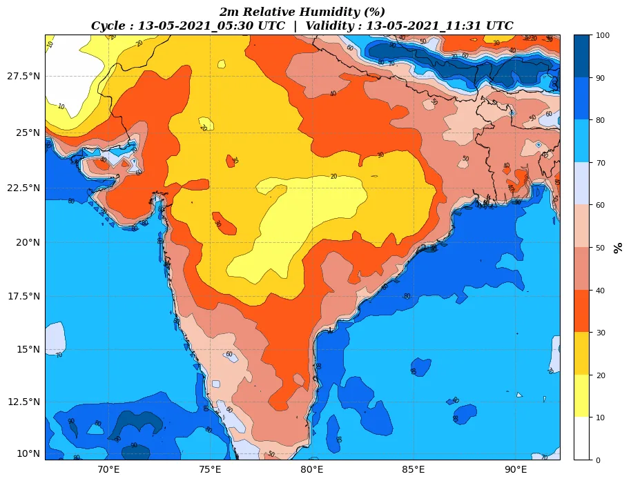
Let’s plot 2m Relative Humidity (rh2):
1
wrfplot --vars "rh2" --input wrfout_d01_2021-05-13_00_00_00 --output ./images
You will see the progress in the terminal along with the location of each image:
1
2
3
4
5
6
7
8
9
*** Initialising plotting for variable : "rh2" ***

        Plotting "rh2" for Time : "13-05-2021_05:30" UTC
          Image saved at : "./images/rh2_13-05-2021_05_30.png"
        Plotting "rh2" for Time : "13-05-2021_08:30" UTC
          Image saved at : "./images/rh2_13-05-2021_08_30.png"
        ...

Plotting process completed. It took 0H:0M:9.682410S
One image is created for every time step available in the file. The output will look like the one shown at the top of this post.
Plot Multiple Variables
You don’t need to run the command again and again for each variable. Just separate them with ,:
1
wrfplot --vars "slp,winds,T2,rh2,ppn_accum" --input wrfout_d01_2021-05-13_00_00_00 --output ./images
Plot Upper Air Variable
Upper air variables are plotted the same way. By default, all the standard levels from 925 to 200 hPa are plotted:
1
wrfplot --vars "u_winds" --input wrfout_d01_2021-05-13_00_00_00 --output ./images
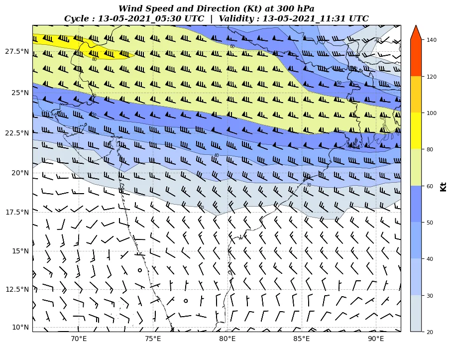 Upper Winds at 300 hPa Plotted by wrfplot
Most of the time, I don’t need all eight levels. You can control it using --ulevels option. For example, to plot only at 850 and 500 hPa:
1
wrfplot --vars "u_winds" --ulevels "850,500" --input wrfout_d01_2021-05-13_00_00_00 --output ./images
The levels should be between 50 and 1000 hPa and separated by ,. It does not have to be one of the standard levels. --ulevels "800,750" works equally well.
Change Colours and Contour Levels
Each variable comes with its own default colour map and contour levels. However, there are times when you want to highlight a specific range. For example, during summer I am more interested in temperatures above 36°C than the full range. Use --clevels for this. Levels are to be in ascending order and separated by ,:
1
wrfplot --vars "T2" --clevels "0,10,20,30,32,34,36,38,40,42,44,46" --input wrfout_d01_2021-05-13_00_00_00 --output ./images
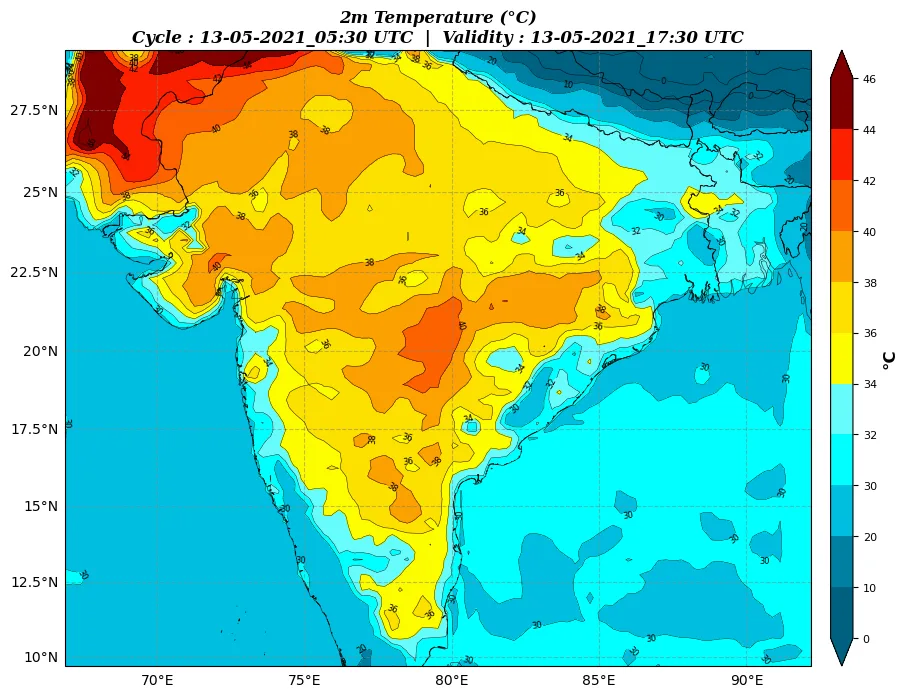 2m Temperature with Custom Contour Levels
If you provide only a single number such as --clevels 10, wrfplot treats it as the number of contour levels (maximum 12) and works out the values automatically. Also note that only whole numbers are accepted at the moment.
To change the colour map, first list the available colour maps:
1
wrfplot --list-cmaps
and then pass the name of your choice with --cmap option. The colour maps come from the excellent colormaps package and you can see how each one looks on its website.
The colour map must have a minimum of 11 colours. Otherwise, it will lead to an error.
If contour labels are cluttering your plot, you can switch them off using --no-clabel option. It has no effect on slp.
Create Animation
This is one of my favourite features. Add --gif to create an animated GIF of all the time steps:
1
wrfplot --vars "rh2" --gif --input wrfout_d01_2021-05-13_00_00_00 --output ./images
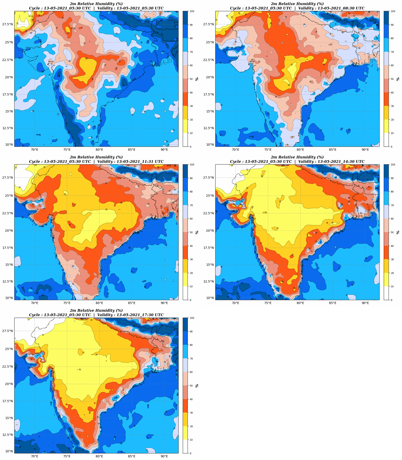 Animated 2m Relative Humidity
The default frame speed is 0.5 seconds. Use --gif-speed to change it. Lower value means faster animation:
1
wrfplot --vars "rh2" --gif --gif-speed 0.25 --input wrfout_d01_2021-05-13_00_00_00 --output ./images
Image Resolution
The default image resolution is 125 DPI, which is good enough for viewing on screen and web pages. If you need images for printing or publication, increase it with --dpi:
1
wrfplot --vars "slp" --dpi 300 --input wrfout_d01_2021-05-13_00_00_00 --output ./images
Remember that higher DPI will also increase the time taken to plot.
Using wrfplot in WRF Run Framework
This is where wrfplot really shines. Since it is a command line application, it can be called from any shell script right after wrf.exe completes. A simple example is given below:
1
2
3
4
5
6
7
8
9
10
#!/usr/bin/env bash

WRF_DIR=/home/sundar/WRF/run
IMG_DIR=/home/sundar/forecast/images/$(date +%Y%m%d)

# Plot surface and upper air products for domain 1
for wrfout in ${WRF_DIR}/wrfout_d01_*; do
    wrfplot --vars "slp,winds,T2,rh2,ppn_accum,mdbz" --input ${wrfout} --output ${IMG_DIR}/surface
    wrfplot --vars "u_winds,u_rh" --ulevels "850,700,500,200" --input ${wrfout} --output ${IMG_DIR}/upper
done
Modify the path and variables as per your requirement. If you installed wrfplot using conda, don’t forget to activate the environment inside the script before calling wrfplot.
What Next?
There are a few options I want to add in future releases:-
--save-format: Save images in different file format other thanpng--titleand--title-font-size: Custom title for the plot
If you find any bug or want a new variable or feature to be added, please raise an issue at https://github.com/wxguy/wrfplot/issues. Pull requests are always welcome.
That’s it for now. I will update this post as and when new features are added to wrfplot.